Data Structure – This is a way of representing/organizing data held in a computer’s memory to be used efficiently.
Data structures fall under 2 categories: Static or dynamic.
Static:
The size is set at the beginning of the program when it compiles and can not be changed. This is very limiting and inefficient as you need to know in advance how large you data structure needs to be. However, static data structures are easy to program and you know how much space they will take up.
Advantages:
The memory allocation is fixed and so there will be no problem with adding and removing data items.
Easier to program as there is not need to check on data structure size at any point.
Disadvantages:
Can be inefficient as memory for the data structure has been set aside regardless if it needs it or not.
Dynamic:
The size does not have a limit but can be more complex to implement. Memory is allocated to the data structure dynamically, as the program executes.
Advantages:
Makes the most efficient use of memory as data structures only uses as much memory as it needs.
Disadvantages:
Because memory allocation is dynamic, it is possible for the structure to overflow if it exceeds its allowed limit.
Harder to program as software needs to keep track of its size and data item at all times.
It is also very common for more complex data structures to be made up of simpler ones. For example, it is normal practice to implement binary trees using a linked list.
Arrays:
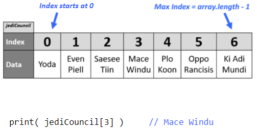
An array is a static data structure which can have multiple dimensions.
One Dimensional:
Each item in the array is assigned an index value starting from 0.
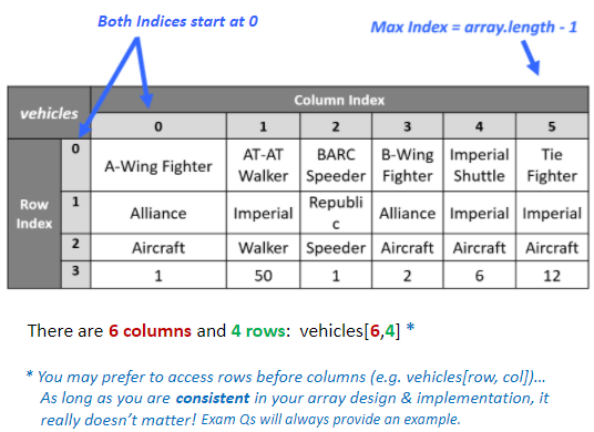
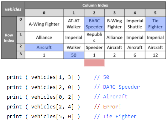
Two Dimensional:
Each item is assigned 2 index values. x and y.
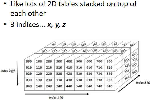
Three Dimensional:
Each item is assigned 3 index values. x, y and z.
Tuples:
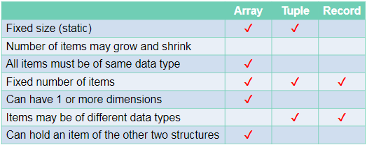
Tuples are very similar to one dimensional arrays but with 2 important differences:
Firstly, tuples cant be edited once they have been assigned (immutable)
Secondly, tuples can contain values of different types unlike arrays where every item must be the same type.
Records:
A record is used to organise data by an attribute.
- They are composed of a fixed number of fields of different data types.
- Can be treated as a tuple.
Stacks:
This is another method for handling linear data lists.
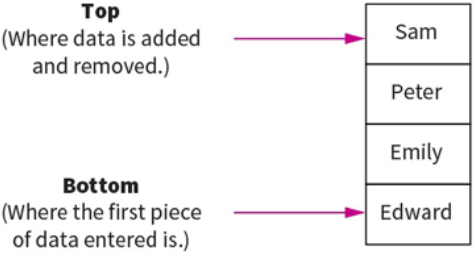
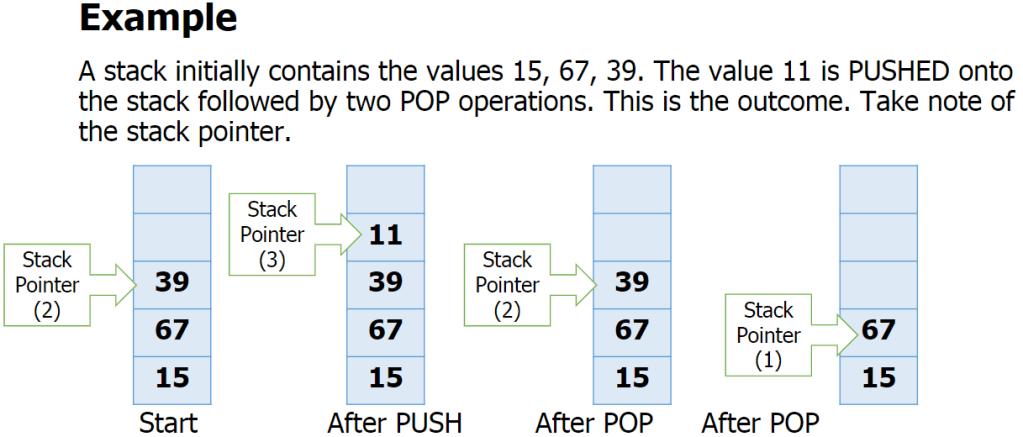
Stacks are last-in first-out (LIFO) data structures. This means that the most recent piece of data added to the stack is the first piece to be taken off it. Meaning to get to the bottom piece of data you need to “pop” out the above data to get to that piece. e.g: teacher puts textbooks on the top of a pile and students take it from the top. Example: like a stack of pancakes.
Adding data to the stack is called pushing and taking data off the stack is called popping.
A stack within a computers memory system is implemented using pointers. The pointer is always pointing to the top item in the stack.
The basic operations for a stack are:
- Adding/removing from the top
- Checking if the stack is full/empty
Basic operations:
push(item) – adds item to the top of the stack
pop() – removes and returns the item on the top of the stack
isFull() – checks if the stack is full
isEmpty() – checks if the stack is empty
also:
peek() – returns top item without removing it.
size() – returns the number of items in the stack
Overflow – attempting to push onto a stack that
is full
Underflow – attempting to pop from a stack that
is empty
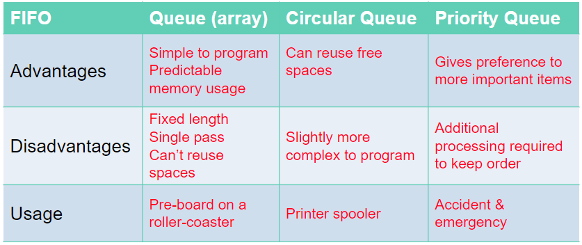
Queues:
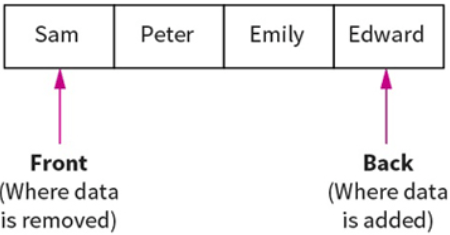
Queues are First In First Out (FIFO) data structures. This means that the most recent piece of data to be placed in the queue is the last piece taken out. Example: At a restaurant, the first person to queue is the first to get their order and leave the queue.
Data within a queue does not physically move forward in the queue. Instead two pointers are used to denote the start and end, to track data items within the structure.
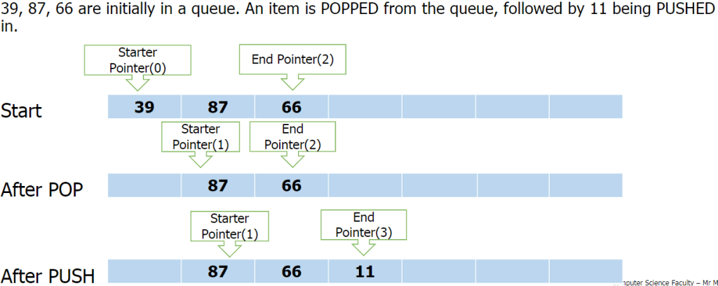
Queue functions/methods:
- enQueue(item) – Add an item to the rear.
- deQueue – Remove and return an item from the front.
- isEmpty – Indicates if the queue is empty.
- isFull – Indicates if the queue is full.
Problems with queue as an array:
- Problems arise with the implementation of a queue as a fixed-size array
- How many items can be added? Or removed?
- What happens when the queue is full, but there are some free spaces at the front?
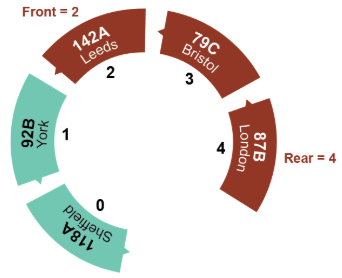
Circular Queue:
A circular queue algorithm overcomes the problem of reusing the spaces that have been freed by dequeueing from the front of the array.
Priority Queue:
In a priority queue some items are allowed to ‘jump’ the queue. Certain items coming in may have some sort of priority to it so it will join the front on the queue.
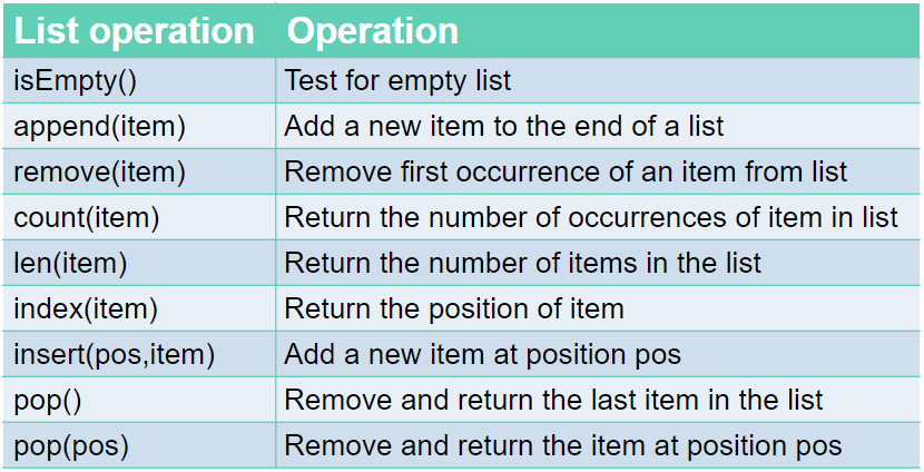
Lists:
Similar to 1D array.
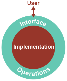
Just like a queue, a list is an abstract data type. An abstract data type, ADT, allows the user to view and perform operations on the data without know how it is implemented/works.
Commands:
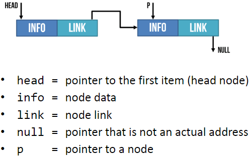
Linked Lists:
Linked lists are one of the most popular type of dynamic data structure. Being dynamic means they can grow whatever size they want.
It is composed of ‘nodes’. Each node is linked to the next node in the list.
Each node is composed of 2 parts: The data and a pointer to the next piece of data in the list.
Adding new data to the end of the linked list you create a new node then you update the last item so it points to the new item.
When searching a linked list, you start at the first node and go through the linked list until the desired value is found or until it reaches the end and it is not contained in the linked list.
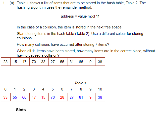
Hash Table:
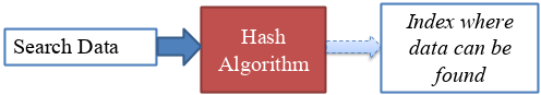
The Abstract Data Structure called a hash table can find any record in the dataset almost instantly, no matter the size of the dataset.
This is done by assigning an address to each data item which is calculated from the data itself using a hasing algorithm. The algorithm uses some part of the record, e.g: the primary key, to map the record to a unique address. The resulting data structure is a hash table.
E.g:
To search for an item you would mod the value and go to the address. If it is not there, go along the table by the skip value until it is found.
There are many other hasing algorithms but they all use the mod function at some point.
When you delete something, it must be replaced with a dummy item such as ‘deleted’. This is because when searching for an item, it keeps looking until it is found or an empty space is found.
The Mid-Square Method:
- First Square the item
- Extract some portion of the resulting digits
- perform the mod function to get an address.
E.g: 562 = 3136
Middle 2 digits = 13
13 mod 11 = 2 = address
The Folding Method:
- Divide the nuber into equal sized pieces (last number may not be equal size)
- Add the pieces together
- Perform mod function to get address
E.g: Store 34721062
34 + 72 + 10 + 62 = 178
178 mod 11 = 2 = address
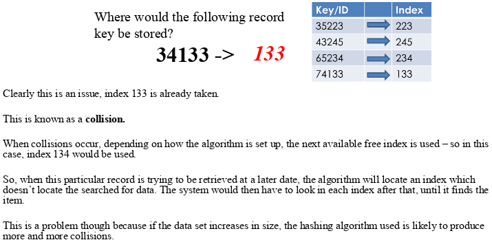
Collosions:
This is when an algorithm generates the same address for different keys. However good the algorithm is, it is impossible to avoid collosions.
To resolve a collision, the simplest method would be to put the item in the next free slot. However, this can lead to clustering in the table. Alternatively, you can increment the ‘skip’ value by adding 1, 3, 5, 7 etc instead of incrementing by 1
Hashing alphanumeric data:
Alphanumeric data may be converted to numeric data by using ASCII code for each character, then applying a hashing algorithm to the result.
E.g: cab
c = 99 a = 97 b = 98
99+97+98 = 294
294 mod 11 = 8 = address.
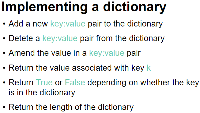
A Dictionary:
A dictionary is an abstract data type made up of associated pairs.
Each pair has a key and a value.
The value is accessed by the key.
A dictionary is a very useful data structure for any application where items need to be looked up.
E.g:
- In a computer, the ASCII
- Translation
Multiple items with the same keys are allowed.
The key:value pairs are not held in any particular sequence. The address of the pair is calculated using a hashing algorithm.
Operations: (In python)
To retrieve a value- dictionaryname[‘key‘]
To insert /update a key-value pair- dictionaryname[‘key‘] = value (when you give a key that is already in the dictionary, it will update its value instead. If it doesnt find the key, it will create a new one.
To remove a key-value pair- del dictionaryname[‘key‘]
To check if a key exists- ‘key‘ in dictionaryname
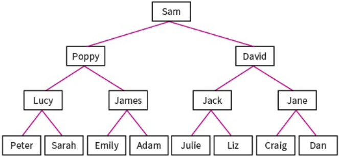
Binary Trees:
Binary trees are composed of nodes, (sometimes called leaves) and links between them (sometimes called branches). Each node can only have up to 2 branches coming from them, often called left child and right child.
Binary search trees are very useful as they have many advantages:
- Trees reflect structural relationships in the data.
- Trees are used to represent hierarchies
- Tress provide an efficient insertion and searching
- Trees are very flexible data, allowing to move subtrees around with minimum effort.
Binary trees are used to implement another data structure called binary search tree. These are identical to binary trees but have the additional constraint that the data on the left branch of a node must be less than the data in the right node. Likewise the data on the right branch of the node must be greater than or equal to the data held in the node.
The RULE: The LEFT node always contain values that come before the root node and the RIGHT node always contain values that come after the root node.
For numeric, this means the left sub-tree contains numbers less than the root and the right sub-tree contains numbers greater than the root. For words, the order is alphabetic. A to left, Z to right.
Example:
Sequnce 20, 17, 29, 22, 45, 9, 19
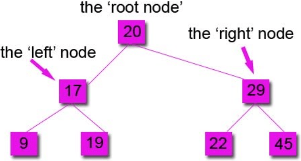
You always compare to the root node first to see if it goes left or right.
Subtracting Nodes:
There are 2 ways to do it:
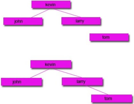
1: Remove the node and move the left node up and attach to the parent node and attach the right node to the right of the left node.
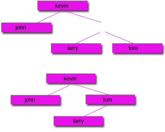
2: Remove the node and move the right node up and attach to the parent node and attach the left node to the left of the right node.
Start with a tree:
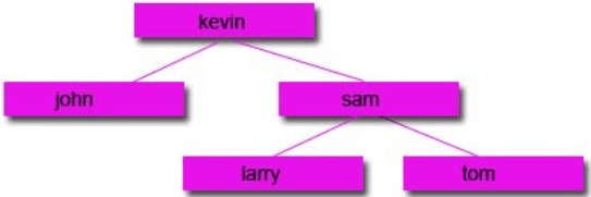
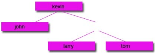
Then remove the node you want:
Option 1:
Option 2:
Traversing data:
Unlike stacks and queues, there is a range of different ways to traverse binary tree data structures. In computer science, traversal refers to the process of visiting (examining and/or updating) each node in a data structure exactly once, in a systematic way. Each method will return a different set of results, so it is important that you use the correct one.
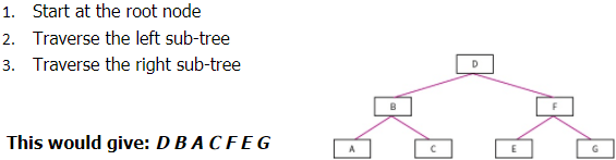
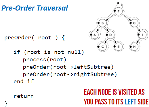
Pre-order Traversal: (Type of Depth First Search)
- Start at root node
- Traverse left sub-tree
- Traverse right sub-tree
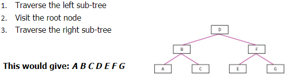
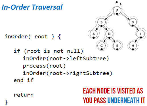
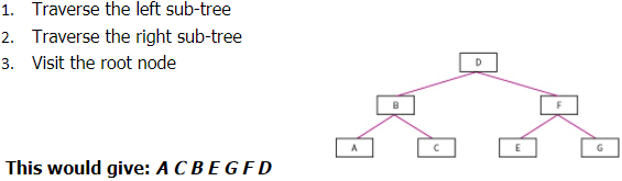
In-order Traversal:
- Traverse the left sub-tree
- Visit the root node
- Traverse the right sub-tree
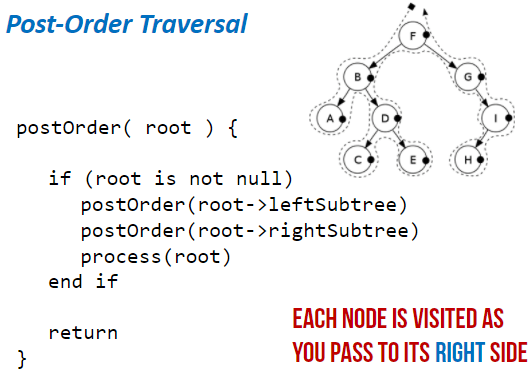
Post-order Traversal:
- Traverse the left sub-tree
- Traverse the right sub-tree
- Visit the root node
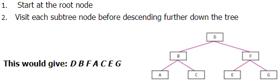
Level-order Traversal: (Type of Breadth first)
- Start at the root node
- Visit each sub-tree node before descending further down the tree
Hash tables:
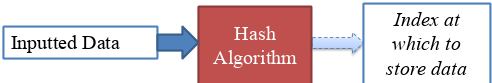
The disadvantages of arrays and linked lists is that if you don’t know the storage location and the data is not ordered, then it can take a while to find the data item. Hashing fixes this. When you enter a data item, a hashing algorithm is applied to the data item and it turns it into the actual index that it will be stored at. This is beneficial because only a simple hashing algorithm is needed so it will be quick and it will give you the exact location of where it is stored in the memory so it will be quick to locate it.
Example:
A database of customers, each record of holding details about a different customer. As it is not known how big the database will become and because data is deleted and added frequently, these record will not be held together in order in the memory. Because of this, locating a record would potentially take a lot of time because we don’t know the index of each record.
To overcome this, a hashing algorithm is applies to each record. This will change it into the index that it is stored at. Now when you search for it, it will apply the hashing algorithm to the search item and it should point to the index of the item.
A common hashing algorithm that is used for 1000 spaces of available memory locations is index = value MOD 1000
Collisions:
This is when the data item is processed through the hashing algorithm and it outputs an index that is already in use. If this happens, the next free index is used.
However, some algorithms deal with collisions differently.
Instead of adding the hashed data to the next available index, it will attach a new array/list to the index and add the data to that. So more than one data item can be placed at the same index but into an array at that index.

This doesn’t help with the time taken to locate the data as once it is searched for, it needs to search the array as well.
When designing a hashing algorithm there are things that need to be aimed for:
- Produce the least possible collisions
- Be as quick as possible. At least faster than another search method.
All data types can be hashed, even strings. This is because each character in a string is in fact an ASCII value. Images can be hashed because image files are in fact a set of pixels which are each stored as a binary number. Sound files can be hashed because sound files are a set of samples which are binary numbers representing frequencies of sound.
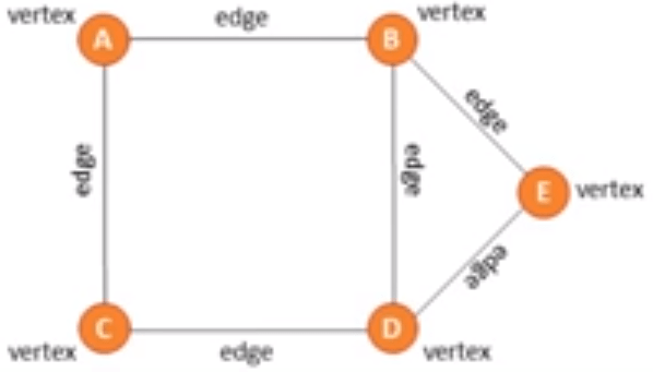
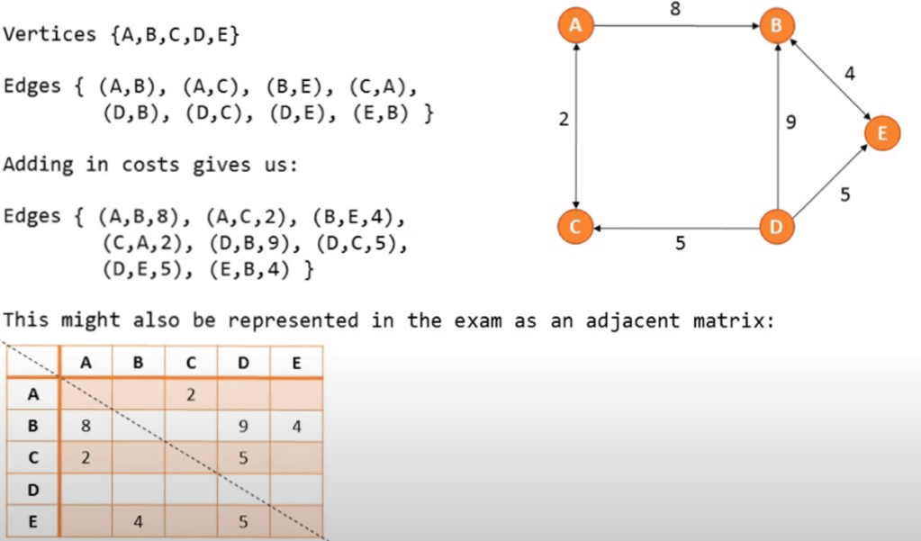
Graphs:
This is a dynamic data structure. It is versatile and is often used in navigation systems, data transmission, web pages and social media trends.
On a graph the nodes are called vertices and the lines are called edges. Edges may be weighted
There are directional and unidirectional graphs.
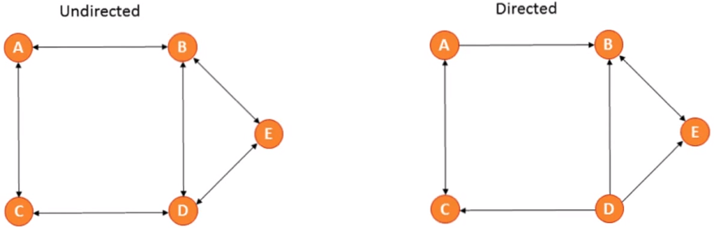
You can represent a graph in 2 ways:
Traversing a graph:
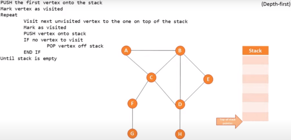
Depth first (using a stack):
Start at the root and follow one branch as far as it will go, then back track.
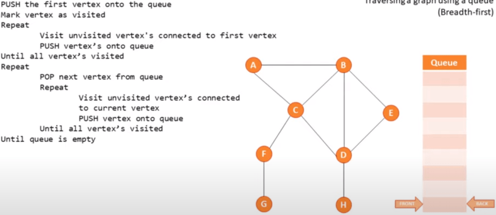
Breadth first (using a queue):
Start at the root, scan every node connected and then continue scanning from left to right.
Pseudo code example: